The compressible Navier-Stokes equations
In computational fluid dynamics (CFD), the Navier-Stokes equations are often solved in an Eulerian, fixed-in-space, frame. Furthermore, it is also convenient to take the fixed frame as being the aeroplane rather than the air, meaning that the object (wing or aeroplane) is at rest and the air is rushing by. The Eulerian form is what I refer to as the compressible Navier-Stokes equations, or just Navier-Stokes equations. The alternative to the Eulerian frame is the so-called Lagrangian, whereby the equations are describing the motion of infinitesimal mass elements of the fluid. These two versions are mathematically equivalent if the velocity field is sufficiently smooth, which is a rather strong assumption. There is also the incompressible Navier-Stokes equations that model, as the name implies, a for all practical purposes incompressible fluid such as water. Since the fluid is incompressible, thermodynamics does not play a role and the speed of sound is «infinite». Mathematically, the equations have a different structure (elliptic-parabolic) than the compressible equations (hyperbolic-parabolic). Here, I do not discuss the incompressible equations, but one should note that the compressible equations should, in some sense, «turn into» the incompressible if the density happens to be constant. The compressible equations are:
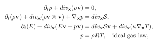
These equations describe the conservation of mass, momentum and energy. rho is the density; v the velocity; p is pressure; S the stress tensor; E the total energy; T temperature; kappa is the heat conductivity coefficient; mu the viscosity coefficient; R is the gas constant.
The hyperbolic continuity equation
Perhaps, the most eye-catching feature of the (compressible) Navier-Stokes equations, is the zero on the right-hand of the continuity (mass) equation. The other equations, conservation of momentum and energy, have diffusive/viscous terms on the right-hand side and the zero breaks this symmetry.
This zero is a real troublemaker. One example has to do with the boundary conditions. For a scalar hyperbolic equation (like the inviscid Burgers equation), an inflow requires one boundary condition and an outflow none. (So-called characteristic boundary condition.) For fully parabolic conservation laws (like the viscous Burger equation), this physically intuitive way of setting boundary conditions is easily generalised. However, the zero in the Navier-Stokes equations destroys this structure in one (subsonic outflow) out of four different flow cases (subsonic in- and outflow and supersonic in- and outflow).
Instead, complicated and rather unintuitive workarounds have to be devised and these do not work well in practice. What does work well, although mathematically incorrect, is to set the physically intuitive boundary conditions as if the system was completely parabolic. In practice, this is what is commonly done.
Another issue that emanates from the zero in the continuity equation appears when attempting to prove well-posedness. Solutions to the Navier-Stokes equations must have non-negative density, temperature and pressure. (This is summarised as «positivity».) For the Navier-Stokes equations positivity can not be proven, without strong a priori stability assumptions. That is, the equations do not guarantee that a valid solution will not evolve into one where positivity is violated. Nevertheless, this is not only a mathematical nuisance; it stands to reason that if a compressible flow model is given reasonable initial data, it does not evolve to an unphysical solution
In fact, negative density or pressure is the most common reason for a CFD code to crash which has spawned research into numerical fixes that prevent this. (See next paragraph.) Nevertheless, it may be argued that a model is not designed to be convenient for mathematical and numerical analysts; it is supposed model the physical reality. However, unless a model is not well-posed, i.e., it is such that for reasonable input data a unique and stable solution exists, predictive simulations are impossible to carry out. Clearly, if a solution does not even exist, the model does not capture the physical reality irrespective of what it was supposed to model and how the model was derived. Although, well-posedness of the Navier-Stokes equations is largely unknown, numerical computations are routinely carried out. However, for non-linear PDEs it is perfectly possible that a consistent numerical approximation of a non-linear conservation law is stable, such that the code produces a numerical solution, that is entirely wrong.
Due to positivity problems one may even argue that it is not the Navier-Stokes equations that are solved in CFD codes. At least not, when the flow is not subsonic, laminar and dynamically stable. In all other cases, substantial artificial diffusion is typically needed in order to stabilise the computations. In particular, artificial diffusion is needed in the continuity equation in order to prevent negative thermodynamic variables. Furthermore, since it is usually impossible to fully resolve realistic flows, these artificial diffusion terms are often larger than the physical diffusion. Hence, it is not the Navier-Stokes equations that are effectively approximated but rather some homogenised Euler system.
There are in fact a number of physically strange properties of the Navier-Stokes equations, that all emanate from the zero in the continuity equation. Namely, there may be a non-zero entropy and energy gradient through an adiabatic wall; relaxation to thermodynamic equilibrium requires convective transport even at the diffusive scale; remarkably complicated (and physically inexplicable) models are required for multi-component flows in order to not violate the non-diffusive continuity equation of the Navier-Stokes equation; based on the constitutive law for Newtonian fluids (Force in x-direction = mu*du/dy) and resistance to compression/expansion (mu*du/dx), it is impossible to interpret all viscous terms that appear as boundary terms on an Eulerian control volume as forces in the direction of the momentum.
Predictive numerical simulations
The design of a numerical scheme through numerical analysis usually follows the same pattern: Find a proof of well-posedness in the literature and then design a numerical scheme that converges to the mathematical solution. That means that one mimics the properties of the solution. The problem is that such a theorem is not available for the Navier-Stokes equations. In fact, proving well-posedess is awarded with a rather hefty lump of money. (As mentioned above, a huge stumbling block is the zero in the continuity equation.)
So, it is unknown what properties numerical solution should have. This may sound as an academic problem but it means that numerical solutions may, or may not, be approximate solutions to the Navier-Stokes equation. This uncertainty is very much is a practical problem.
Today, useful engineering CFD is often carried out by teams of scientist and engineers. Apart from the numerics and physics, it takes experience and technical skills to produce good computational grids and production CFD codes must run fast on parallel (nowadays often heterogeneous) machines, which calls for the skills of computer scientists. Through validation and testing, a computational tool can then be developed. When running a new problem that is similar to the validation cases, the result can be trusted with a reasonable confidence. However, the more the problem is changed, the less the results can be trusted. Ideally, if a model (the set of equations) has been validated, then any provably convergent code (be it finite difference, discontinuous Galerkin, spectral element or any other method) should produce reliable solutions to any aerodynamic problem as long as it is computationally feasible.
Aerodynamic computations typically require the use of very large grids and are thus very expensive (requires massive computational power) and time consuming. Although, one may need to run a few simulations, with slightly different input, to assess the sensitivity of the problem, it is unfeasible to run it 100s or 1000s of times to obtain statistical data from which a solution is built. The output of a single run has to represent the solution, in some reasonable way (but perhaps not pointwise). For instance, the averaged velocity in some small region of a turbulent flow should accurately represent the mean velocity in that area, although the smallest eddies may be inaccurate. Mathematically, this calls for rather strong notion of well-posedness. Today, such theory seems far away for the Navier-Stokes equations.
Although, there are a number of issues with the Navier-Stokes equations, fact remains that it has been very successful in modelling compressible flows since they are derived from sound physical reasoning. However, it is also a fact that these equations are not fundamental in the same way as other equations in physics. They are not derived exclusively from first principles. It is tempting to speculate that for other, less canonical equations, such huge mathematical difficulties would have prompted scientists to explore other paths.
It should be duly noted that there has been research into modifications of the standard Navier-Stokes equations (e.g. by Brenner and more recently by many other scientists), but most often modifications are aimed to improve the physical validity range of the Navier-Stokes equations rather than resolving any well-posedness issues. Somehow, lack of well-posedness is not perceived to be a huge disadvantage of the model. An equally capable, but well-posed model, is consequently not considered to be of much value. Of course, one can also argue that the Navier-Stokes equations have been extensively validated. While this is true, it is generally less true than often assumed by CFD scientists. It is not that computational and experimental data line up on top of each other in all cases. Furthermore, there is a plethora of different models for e.g. viscosity and heat conduction that gives some wiggle room to choose the model best suited for the particular experiment. It would surprising if other compressible flow models derived from similar physical assumptions would not do as well.